Value Study of GLAMs In Canada
Report for the Ottawa Declaration Working Group
Appendix 1 Economic Welfare Approach
Theoretical Framework
This report uses what is known as an economic welfare approach in order to undertake a CBA for the GLAM sector in Canada. CBA has often been employed for the appraisal of major social initiatives, such as new infrastructure or health projects but, as discussed below, extensions of the approach are increasingly being employed in areas such as the environment and the arts.
Of key importance in assessing value under this sort of approach is the assessment of consumer ”willingness to pay” ( WTP) for a given good or service.
For example, in this case, if visitors to GLAMs placed a value on their visit only just equal to the cost of getting there (in time and money), then what they spend and receive would be equivalent and they would be indifferent between visiting and not visiting. In practice, they visit because what they are willing to pay for the experience exceeds the costs of the visit. So, they evidently see visiting as “worth it.”
In economic welfare, the difference between what people do pay and the maximum they are willing to pay is known as their “consumer surplus.” So, a visitor may pay $20 in travel and time costs to get to a GLAM but enjoy it so much that he or she would have been prepared to visit, even if it cost $30. The consumer surplus for such a person would be $10. If a second visitor also experiences costs of $20 to get to the GLAM but is only willing to pay $25 to visit, his or her consumer surplus would be $5.
In this way, consumers enjoy benefits over and above the prices they actually pay. A similar dynamic can be seen on the producer’s side. The “producer surplus” is therefore the difference between the revenue received by the producer (in this case GLAMs) and the minimum they would have been able to produce these services for. Roughly speaking then, producer surplus equates to the producer’s profits.
Fig. 31 below illustrates these concepts graphically. When the price of the thing being valued (for example, the cost to get to a GLAM) is P, the consumer surplus is identified by the area shaded in dark blue, which represents the sum of all these individual visitors’ consumer surpluses. This is the difference between the maximum those visitors would be willing to pay and the amount they actually pay. The latter defines a demand curve, which traces the number of visitors that would be expected given differing access costs.
Consumer surplus may also arise from other forms of interaction with GLAMs, such as usage of their online services and social media as discussed in Chapter 6.
Similarly, the producer surplus (the light blue area) represents the difference between the revenue received by the producer and its operational and maintenance costs.
In the case of GLAMs though, the sector as a whole does not produce a profit in the conventional sense. However, it is still necessary to include its commercial revenues (e.g. earned through admissions, shops, cafes, etc.) as these represent a source of value to be set against the costs of running the organizations.
Adding up the producer and consumer surpluses that flow from a good, program or initiative provides a measure of its benefits. In addition, there may be benefits to third parties (“externalities”) arising from GLAMs’ activities. For example, school trips may develop learning and educational skills, boosting participants’ “human capital.”
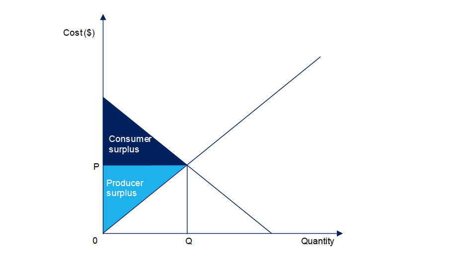
Figure description
The sum of all of these benefits can be compared to the costs of the initiative to produce a BCR. A BCR divides benefits by costs; a BCR greater than 1.0 indicates that an initiative provides a net benefit to society.
Total Economic Value
The above approach is often employed when estimating the value of commodities traded in markets, along with an allowance for some externalities. However, in recent years economists have broadened these ideas to develop what is known as a Total Economic Value framework ( TEV).Footnote 114
A TEV provides an expanded concept of externalities. It recognizes that institutions like GLAMs may be valued not only through their direct “use value” to society, but through a variety of “non-use” (or “passive use”) values. These include existence value (the value placed on the fact that GLAMs exist even though the person in question never uses them), bequest value (the value of preserving GLAMs for future generations), and option value (having the option of using GLAMs, whether or not a person ever chooses to do so).
This study uses a TEV framework for its assessment of the GLAMs sector. The figure below indicates the various components of use and non-use value adopted for this study. These sources of value are then compared to costs to develop a BCR for the sector.
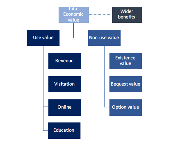
Figure description
Physical and Temporal Scope
In some cases, a “ringfence” is applied to limit the scope of a CBA or TEV. For example, studies may limit the analysis of costs and benefits to a province or a country, such as Canada. People and entities to which an assessment is restricted are known as the “population of standing.”
In the case of the current analysis, no ringfence has been applied. That is, no distinction has been made between Canadian and foreign users of GLAMs (e.g. tourists visiting GLAMs, foreign users of GLAMs websites). Benefits accruing to all of these parties are therefore considered within the framework of the analysis, though most of the costs are borne by Canadian society (e.g. government subsidies to maintain GLAMs).
Another scoping issue relates to time. As the objective here is to appraise the impact of a single year of GLAMs’ operations, the current year used in this study is assumed to be 2019. Accordingly, this assessment generally matches current costs, expressed in 2019 prices, with the benefits enjoyed during that year.Footnote 115
In the case of the assessments for education and student use of academic libraries, however, the bulk of the benefits occurs in the future, but nonetheless arises out of costs incurred in the present. Accordingly, these benefits have been measured over future years on a present value (PV) basis. A PV approach adds up benefits enjoyed in future years, subject to discounting to allow for the fact that future benefits are worth less than current ones. Another way of viewing this approach is that all benefits associated with costs incurred in the present are effectively measured on a PV basis, but are greater than zero only in the case of education and academic libraries. This is because other forms of benefits (e.g. physical use value) cannot be realized in future years without future expenditures.
Appendix 2 Valuing Glam Visits
Approach
As indicated in Chapter 4, travel cost models for various GLAMs were estimated using a combination of “bottom up” TCMs gathered from various GLAMs across the country, and the results of our national survey, which produced “top down” perceived cost measures. The average of the bottom up and top down estimates was used to derive the final values for consumer surplus for the various GLAMs.
Bottom Up Institutional Travel Cost Models ( Tcms)
The starting point for our bottom up analysis was the detailed information on postal code of residence gathered by various GLAMs from their visitors at the point when they purchased a ticket or requested a service.Footnote 116 While all visitors to GLAMs were included in the analysis, for the purposes of assigning travel and time costs in our travel cost models, a “day trip” cost boundary of 250 kilometres from the relevant institution was set. Trips originating within this boundary were assigned to zones as described below. Trips originating from outside the boundary were assumed to have a similar pattern of trips to those inside it and assigned to zones within the boundary accordingly.Footnote 117
To obtain an estimate for the value of GLAMs to their visitors, we then worked through the following steps:
- We matched the postal codes identified in the institutions’ data with the Forward Sortation Areas ( FSA) used in Statistics Canada population data.
- For each FSA in our dataset we estimated the distance to the institution under consideration based on a Google maps algorithm.
- We aggregated FSAs into 10 zones based on the distance from the GLAM under consideration. Using population data for the FSAs within each zone and the number of visitors identified in our dataset we could establish a visit rate to the GLAM for each zone. For example, if 200,000 visits to a museum came within 10-20 km driving distance, and the total population in this zonal bracket was one million, then the visit rate per thousand population would be 200.
- To determine the time travelled by visitors from each FSA, we used the same Google maps algorithm described above. Since we needed a single travel cost and time for each FSA, we made some assumptions on the transport mode. These assumptions were designed to align as closely as possible with the results from our national survey of the general Canadian population.
- To capture the full cost of a visit it was necessary to calculate the true direct travel costs—taking account of fuel consumption and other vehicle costs, or transit fares—as well as the “opportunity cost” of the time spent travelling.
- The next step was to identify the demand curve implied by the rate at which visits to GLAMs fell as travel costs increased. It is important to recognize that this is a non-linear relationship, with visit rates falling at a slower rate at greater distances from the GLAM. Taking the natural logarithm of visit rates and travel costs produced a linear relationship from which we could estimate a statistical relationship between visit rates (VVrr) and total individual costs (TCC) using ordinary least squares, as shown in the equation below:
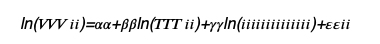
Fig. 33 below shows an example plot of this model (Royal BC Museum data), which suggests a good fit of the data, exhibiting an R squared of 91%. The travel cost coefficient is negative and highly significant. - The results of this regression determine the relationship between costs and visit rates in the abstract, allowing us to simulate the likely number of visitors should the entry fee to the GLAM be raised by any given amount. Simulating visitor numbers at a variety of new entry fees traces the full demand curve, giving the consumer surplus as the area under the curve, as shown in Fig. 34.
- GLAMs’ data suggest that a small number of people would be prepared to incur large costs to visit them. Since large expenditures begin to look implausible, when calculating consumer surplus, we truncated the demand curve at $200. This provides a more conservative estimate of consumer surplus.
- The consumer surplus is calculated as the area under the demand curve. Dividing the resulting total by the total number of visits in the sample produces the average consumer surplus per visit.
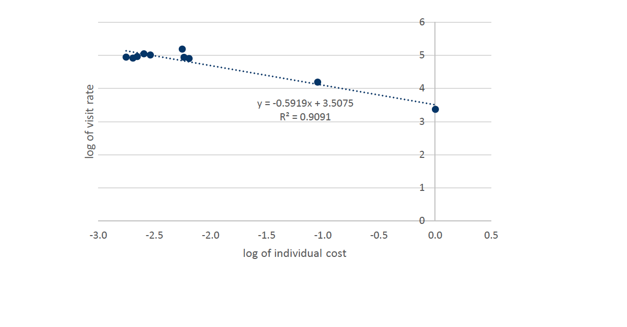
Figure description
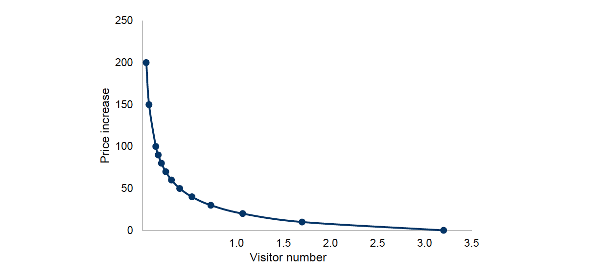
Figure description
Source: Oxford Economics
Top Down Tcms
The top down TCMs used data gathered through our national survey. In the case of archives, this was supplemented by data gathered by Yakel et al (2012). An anonymized version of the origin-destination data from this study was kindly provided to us by Professor Wendy Duff of University of Toronto.
The survey included questions about whether respondents had used a GLAM in the previous year. If so, they were asked to nominate how much time and money they spent on the most recent visit to that institution.Footnote 118 This allowed us to develop separate “supermodels” (national models) for galleries, libraries, archives and museums using a TCM approach, as described below. The methodology was similar in its broad outlines to the bottom up approaches, though with some important differences. The approach was as follows:
- The estimated (one way) cost of travel was directly provided by respondents.
- The (one way) time taken to reach the institutions was also directly provided. This was monetizedusing the Canadian values of recreational time described in Chapter 4 ($13.7/hour). In the caseof libraries and archives, the average time cost was a mix of recreational time and work time, assome users were there for work purposes (21% for libraries, 27% for archives). This producedvalue of time estimates of $16.6/hour for libraries and $17.4/hour for archives.
- The one-way trip costs were then added up and doubled to reflect the cost of two-way trips.
- As indicated these costs reflected perceived costs of the journey and perceived time taken tocomplete the trips, as opposed to the researcher defined costs in the bottom up models.
- In the case of the archival data, using the information from Yakel et al., the base data consistedof usable origin-destination points for 468 trips across the nation. We then used the Google Mapsalgorithm from the bottom up model to determine distance and travel time by transport mode, andthen used these as the basis for travel costs.
- As was the case with the bottom up models, demand curves were estimated using a double logapproach, although data limitations meant that only total individual costs ( TC) were employed asexplanatory variable (i.e. income was excluded). In addition, admission prices were not explicitlyincorporated into the national models, though these may be only a relatively modest part of totalcosts.Footnote 119 Nonetheless, all specifications returned relatively high R2 indicating good model fit.
- As is the case with the bottom up models, the results of this regression determine the relationshipbetween costs and visit rates in the abstract, allowing us to simulate the likely number of visitorsshould the entry fee to the GLAM be raised by any given amount. Simulating visitor numbers at avariety of new entry fees traces the full demand curve, giving the consumer surplus as the areaunder the curve.
- The consumer surplus is calculated as the area under the demand curve. Dividing the resultingtotal by the total number of visits in the sample produces the average consumer surplus per visit.
- As is the case with the bottom up models, since large expenditures begin to look implausible,when calculating consumer surplus, we truncated the demand curve at $200 (with the exceptionof libraries where it was truncated at $125). This provides a more conservative estimate of consumer surplus.Footnote 120
We have given an example of the demand curve from the national model for museums below. The equation indicates the relationship between visitation (LnV) and travel costs (LnP) (expressed in logs). This form of model, known as “double log,” allows us to determine the responsiveness of visits to price in percentage terms. The coefficient on travel costs (-0.78) indicates the elasticity or responsiveness of museum demand to price. In other words, for every 1% increase in the cost of getting to museums, the number of visits falls by 0.78%.
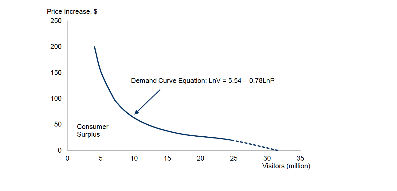
Figure description
As suggested above, based on the national models it is possible to provide estimates of the elasticities (or responsiveness) of users to the costs of accessing GLAMs. This provides a hint of how much changes in access price might affect usage.
Elasticities over 1.0 are said to be price elastic—e.g. a 1% change in price would generate a greater than 1% change in demand. Elasticities below 1.0 are said to be inelastic—e.g. a 1% change in price would be accompanied by a smaller than 1% change in demand.
Elasticities can be affected by the uniqueness of the resource in question, the preferences of the group and/or the presence of alternatives. For example, the elasticity of 1.06 for libraries may be indicative of the fact that there are several alternatives to library usage if access prices get too high (e.g. borrowing from friends, buying). The elasticity of 0.55 for archives could reflect the uniqueness of physical archival resources and the determination of a smaller number of users to access them even if costs are high.
Likewise, the elasticities can tell us what would happen if prices rose (or fell) in real terms (i.e. after allowing for inflation). So, for example, according to the model results, a 10% increase in the cost of accessing archives might be met with only a 5.5% decrease in demand. But a 10% increase in the cost of library access would be met with a 10.6% decrease in demand.
We have also provided some key model diagnostics in Fig. 36.
| Item | Galleries | Libraries | Archives (Yakel et al data) |
Museums |
|---|---|---|---|---|
| Elasticity | 0.81 | 1.06 | 0.55 | 0.78 |
| T statistic | 16.5 | 31.1 | 56.2 | 19.8 |
| Model R2 | 0.86 | 0.94 | 0.91 | 0.87 |
| Number of respondents (n) | 204 | 826 | 468 | 253 |
Source: Oxford Economics
All figures subject to rounding.
Final Results
As indicated, the bottom up approach pooled results from a number of institutions across the country, while the top down approach utilized the national survey data (or, in the case of archives, the Yakel et al. national data).
In addition, the bottom up approach used institutional data and combined this with estimates of the time, distance and ultimately costs faced by GLAMs users.Footnote 121 So the approach used what is sometimes called objective or researcher defined costs—i.e. the costs were estimated by the analysts. With the exception of the archives’ model, the top down approach used respondents’ own estimates of the time taken and distance travelled—i.e. perceived costs.
Researcher defined costs may appear preferable as they seem more objective and less subject to bias, but debates continue around this issue.Footnote 122 This is because demand curves are effectively the product of perceived costs. So if users truly feel that a GLAM visit took, for example, more time and money than the “objective” costs suggest, their valuations and number of visits will reflect that. In addition, the national models may give a more comprehensive picture of user costs across many institutions, nationwide, than the bottom up modelling approach.
There are no “right” or “wrong” answers to this issue. We have taken a middle path in this analysis by taking the average of the pooled bottom up consumer surplus per trip values and the top down models. The final consumer surplus estimates using the average of these two approaches are indicated in Fig. 37.
| Item | Galleries | Libraries | Archives | Museums |
|---|---|---|---|---|
| Consumer surplus per trip– final estimate (CAD) |
44 | 18 | 65 | 44 |
Source: Oxford Economics
All figures subject to rounding.
Appendix 3 Online Value
Approach
As indicated in the main text, the time users spend online accessing GLAMs’ websites, catalogues and social media portals provides one indication of how much people are willing to give up to access GLAMs’ content. This can be used to develop the online equivalent of TCMs in some ways.
Work by Goolsbee and Klenow (2006) and Pantea and Martin (2014) was used as a “mathematical road map” to estimate a demand curve and CS for online activity.Footnote 123 The estimate of elasticity (responsiveness) to the cost of time online (1.6 as detailed below) was then used to estimate the consumer surplus for online users.
Details
Work by Goolsbee and Klenow on the value of the Internet indicates that time spent online can be combined with an estimate of leisure demand elasticity to derive a “linear demand” estimate of online consumer surplus. This would form a lower bound value for consumer surplus.Footnote 124
Examining the Goolsbee and Klenow work suggests an elasticity of leisure demand of 1.6. That is, for every 1% increase in the amount of time taken to access a given amount of information on a GLAM website, user demand falls by 1.6%.
However, these authors note that this linear approach represents a lower-bound estimate, with a log demand model suggesting values 3.8 to 9.2 times higher than those produced by the linear model. Subsequent authors have also undertaken quantitative work, which suggests that Goolsbee and Klenow’s linear consumer surplus estimates are likely to be much too low.Footnote 125
Calibrating the results of Goolsbee and Klenow’s work with later authors, such as Pantea and Martin (who analyzed European Internet elasticities), suggests that values derived through the upper bound are probably in the close to the minimum log to linear model ratio examined by Goolsbee and Klenow (3.8).
Data on the number of website visits to GLAMs is available through Canadian Heritage, while data on large public libraries’ online sessions is available through CULC.Footnote 126 There is no equivalent comprehensive information on social media portal usage, so social media usage was estimated from the national survey data, as described below.
Data on the time spent on GLAMs’ websites form the starting point for an estimate of the consumer surplus enjoyed by their users. The national survey included questions on the time spent online using websites and social media portals of individual GLAMs and the frequency of such usage. Social media portals examined included Facebook, Twitter and Instagram.Footnote 127
In addition, data was sought from GLAMs across Canada on usage of websites and/or social media, as a consistency check on the survey results.Footnote 128
The average session time on GLAMs’ websites ranged from 24 to 35 minutes according to the national survey results, whereas the average session times reported by available GLAMs institutional data typically ranged from roughly 2 to 6 minutes.Footnote 129
In considering this and the other issues above, there are a number of upward and downward factors which could impact on the assessment of online benefits:
- Linear vs logarithmic model—Using a log model would constitute an upper bound estimate for the consumer surplus valuation, while using a linear approach would produce a lower bound estimate. So, a linear model could bias results downwards while a log one could bias them upwards.
- Survey vs reported session times—As indicated, the average survey session times reported in the national survey were considerably greater than the session times reported by individual GLAMs. One reason for this can simply be that users “got it wrong” and overestimated the time spent online. If so, using survey average times would bias results upwards. However, the national data are comprehensive, whereas the institutional data are limited to reporting institutions, and session times vary depending on the type of institution. More fundamentally, neither time measure may be “wrong.” The issue here may be similar to that of perceived versus researcher defined costs for the TCMs. Demand curves are built on perceived costs, so if users perceive they are sacrificing this much time online, this will define their demand curves and valuations, rather than the “objective” session time recorded by institutions.
- Coverage of social media portals—As indicated, coverage was limited to Facebook, Twitter and Instagram due to sample size issues with the national survey. While the small samples sizes themselves indicate much lower usage of these portals, the omission of other portals would bias results downwards.
- Leisure time versus work time—The elasticity estimation (1.6) represents a leisure elasticity. However, some of the time spent on libraries’ and archives’ websites is work time. If that is the case, online demand for those institutions may also be less elastic. Applying a constant elasticity of 1.6 could therefore bias results downwards for those institutions.
In balancing these considerations, we have used the national survey median session times as the basis for the amount of time spent on GLAMs’ online channels. Median times are lower than average times, ranging from 15 to 20 minutes for websites and 15 to 23 minutes for social media portals. This recognizes that perceived time costs may be relevant to valuations, while taking into account data from individual GLAMs, suggesting that average session times might be subject to overestimation. We have also adopted a linear (i.e. lower bound) model to help ameliorate any issues with overestimation of session time in the national survey. As there remains some potential for downward bias from some of the other factors described above, our online value estimates may be on the conservative side.
Data on website sessions’ number and duration described above were combined with information on the value of leisure time ($13.7 per hour, as derived for the TCMs). Social media usage was estimated based on national survey results. In the case of libraries and archives, an allowance was also made for proportion of time that was work related, based on the physical usage statistics derived for the TCMs (21% for libraries and 27% for archives).
The figure below provides an illustration of how the estimation process worked in the case of museums websites. The process takes the data above and uses the fact that consumer surplus can be estimated using elasticities.Footnote 130 Given an estimated time cost of $3.42 per session, 89.5 million annual website sessions and an elasticity of 1.6, this suggests a consumer surplus of $95.7 million for museum websites alone. A similar approach was adopted for other GLAMs’ websites, catalogues and for social media.
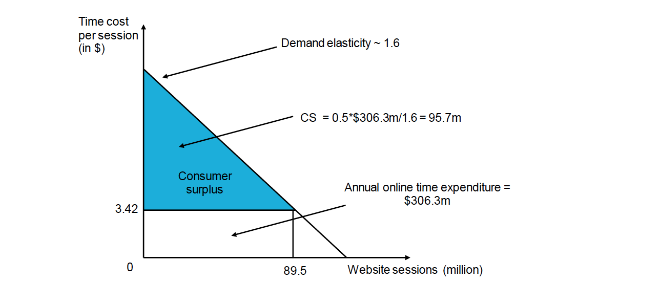
Figure description
An additional note to the above discussion is that the data collection process suggests that there is little information about the usage of social media data by GLAMs users. The survey may help addressing such issues though, as noted, coverage was incomplete due to sample size issues.
Appendix 4 Wider Benefits: Wellbeing
Approach
As indicated in Chapter 8, two approaches were utilized in undertaking quantitative modelling of wellbeing. These were:
- Approach 1—the relationship between those who used GLAMs during the past year and wellbeing (the usage approach); and
- Approach 2—the relationship between frequent (three or more times) GLAMs users and wellbeing (the frequency approach)
Both of these approaches are discussed in more detail below.
Modelling Methodology: Usage Approach
Under Approach 1, those who used GLAMs during the past year (i.e. current users) were separated out from those who did not, using our national survey data. As indicated in Chapter 8, a series of regressions were run to try to determine if GLAMs usage was related to improvements in various measures of wellbeing explored in the national survey (i.e. subjective wellbeing, health, neighbourliness, and volunteering).
The wellbeing measures draw off the questions reported in Questions G4-G7 in the national survey (see Appendix 6). These questions were based on those used in past surveys such as Statistics Canada’s General Social Survey, 2010 Cycle 24 – Time Stress and Well Being. Many things can affect a person’s wellbeing; for example, people on higher incomes might be healthier (or indeed their superior health might help them earn a higher income). Accordingly, to help tease out the importance of GLAMs usage on wellbeing, the regressions also used demographic information collected in the national survey and controlled for other factors such as income, age, education and employment status.Footnote 131
Consistent with the approach taken in recent wellbeing research, a series of ordinary least squares (OLS) regressions were run to determine the impact of GLAMs usage on various wellbeing indicators.Footnote 132 The wellbeing states were specified as dependent variable (i.e. the variable being measured) whereas the independent variables (i.e. the factors that might affect the dependent variable) were GLAMs usage, disposable income (logged), age, education and employment status. Apart from income, the independent variables were specified as categorical variables (i.e. variables used to distinguish between different groups). This is consistent with the use of categories to distinguish different groups (e.g. employed, unemployed) in the national survey.
| Variable | Description | Coding |
|---|---|---|
| Health | Self-assessed health rating | Scale of 1-5 where 1= poor and 5 = excellent. (Dependent variable) |
| Neighbourliness | Know neighbours | Scale of 1-4 where 1 = know no neighbours and 4 = know most neighbours (Dependent variable) |
| Volunteering | Volunteered in last 12 months | Scale of 1-2 where 1= Have volunteered in last 12 months and 2 = Have not volunteered in last 12 months (Dependent variable) |
| Current User GLAMs | User of at least one GLAM in the last 12 months | 1 if Yes, 0 if No (dummy variable) |
| Current User Galleries | Visited galleries in last 12 months | 1 if Yes, 0 if no (dummy variable) |
| Current User Libraries | Visited libraries in last 12 months | 1 if Yes, 0 if no (dummy variable) |
| Current User Archives | Visited archives in last 12 months | 1 if Yes, 0 if no (dummy variable) |
| Current User Museums | Visited museums in last 12 months | 1 if Yes, 0 if no (dummy variable) |
| Disposable income | Disposable income | Log of disposable income |
| Degree | Have a degree | 1 if have a degree, 0 otherwise (dummy variable) |
| Employed | Employed full time or part time | 1 if employed full or part time, 0 otherwise (dummy variable) |
| 15-24 | 15-24 years old | 1 if 15-24, 0 otherwise (dummy variable) |
| 65+ | Over 65 years old | 1 if 65 or over, 0 otherwise (dummy variable) |
| Gender | Male, female or other | 1 if Male, 0 if Female (dummy variable) (no “other” responses received) |
An “At Least One GLAM” (ALG) model was run, examining whether the usage of at least one GLAM during the past year was related to an improvement in wellbeing. In addition, separate models were run examining how usage of each individual institution affected wellbeing.Footnote 133
No statistically significant relationship was found between GLAMs usage and subjective wellbeing. However, as indicated in Chapter 8, there may be a variety of reasons for this, and wellbeing may be distinguished from happiness. Health states, in turn, may be a lead indicator—if not a proxy for—happiness. Given this and recent Canadian initiatives recognizing the relationship between GLAMs and health visitation (e.g. writing prescriptions for visits to the Montreal Museum of Fine Arts), the health regressions are of particular interest. These are indicated below.
| Variable | Coefficient |
|---|---|
| Ln of Disposable Income | 0.28* |
| Current user GLAMs | 0.14* |
| Degree | 0.16* |
| Employed | 0.22* |
| 15-24 | 0.44* |
| 65+ | 0.18* |
| Male | 0.00 |
| _constant | - 0.09 |
| R2 | 0.09 |
Source: Oxford Economics analysis
*Significant at the 5% level
| Variable | Coefficient |
|---|---|
| Ln of Disposable Income | 0.27* |
| Current user galleries | 0.13* |
| Degree | 0.16* |
| Employed | 0.23* |
| 15-24 | 0.43* |
| 65+ | 0.19* |
| Male | 0.00 |
| _cons | 0.05 |
| R2 | 0.09 |
Source: Oxford Economics analysis
*Significant at the 5% level
| Variable | Coefficient |
|---|---|
| Ln of Disposable Income | 0.28* |
| Current user of libraries | 0.13* |
| Degree | 0.16* |
| Employed | 0.23* |
| 15-24 | 0.44* |
| 65+ | 0.18* |
| Male | 0.01 |
| _cons | 0.11 |
| R2 | 0.09 |
Source: Oxford Economics analysis
*Significant at the 5% level
| Variable | Coefficient |
|---|---|
| Ln of Disposable Income | 0.27* |
| Current user of libraries | 0.22* |
| Degree | 0.18* |
| Employed | 0.23* |
| 15-24 | 0.43* |
| 65+ | 0.19* |
| Male | - 0.01 |
| _cons | 0.02 |
| R2 | 0.09 |
Source: Oxford Economics analysis
*Significant at the 5% level
| Variable | Coefficient |
|---|---|
| Ln of Disposable Income | 0.27 |
| Current user of libraries | 0.10* |
| Degree | 0.16* |
| Employed | 0.23* |
| 15-24 | 0.45* |
| 65+ | 0.18* |
| Male | - 0.00 |
| _cons | 0.01 |
| R2 | 0.09 |
Source: Oxford Economics analysis
*Significant at the 5% level
These regressions indicate that GLAMs usage is associated with a statistically significant increase in health states.Footnote 134 For example, gallery visitation during the past year was associated with a 0.13 point higher reported health state (on a scale of 1-5), compared to non-users. Of course, these regressions also tell us about the impact of other variables—e.g., using the galleries model again, having a university degree is also associated with a 0.16 point higher reported health state than those who did not have one.
Correlation does not prove causation. For example, GLAMs may improve people’s health—or perhaps more healthy people are the ones who visit GLAMs. Nonetheless, analysts such as Fujiwara contend that the various demographic controls in similar model specifications help support the case for GLAMs having positive effects on wellbeing.Footnote 135
Moreover, as discussed in much of the wellbeing and “happiness economics” literature in recent years, these values can be monetized to provide an indication of how much visiting GLAMs is equivalent to in terms of wellbeing. What is essentially being measured is the effect of GLAMs on wellbeing and the monetary equivalent of that. For example, if visiting GLAMs increases self-reported health (and, thereby wellbeing) by 1 point, and $1,000 in income also increases self-reported health by 1 point, then the equivalent value of using GLAMs is $1,000 in improved wellbeing. The technical name for the effect on wellbeing is the “Compensating Surplus.”Footnote 136
We have used the ALG model to provide a broad indication of how GLAMs visitation might be valued using such a wellbeing approach. The approach to doing so followed the established literature in the field and was as follows:
- The relationship between the ALG usage coefficient (0.14 for all GLAMs) and the income coefficient allows for an estimation of the effect of GLAMs visitation expressed in Canadian dollars.
- This approach uses the fact that income is expressed in monetary terms and the fact that the equation coefficients report the relative sizes of these factors ( GLAMs and income) on health (the dependent variable). So, if income does indeed improve health (and, by doing so, happiness), then, as suggested above, the relationship between the size of the income coefficient (0.28) and the size of the usage coefficient (0.14) gives us a clue of the effects of GLAMs usage on wellbeing, as expressed in monetary terms.
- This can be further adjusted to deal with health-income causality (i.e. good health could cause income to be higher or vice versa). Ideally this could be done by using an “instrument” for income. However, where this is lacking, Fujiwara suggests inflating the income term by a factor of 2-10.Footnote 137 We apply a factor of 10 (i.e. the most conservative value) and use this to multiply the income coefficient to control for reverse income causality.
- Given a logged income term, this relationship can be expressed as Compensating Surplus = M0 – e[ln(M0)-β2/ β1] where M0 is median disposable income estimated based on the national survey results ($29,855), β1 is the adjusted income coefficient (2.75) and β2 the usage coefficient (0.14).Footnote 138
- Applying this equation, we derive a monetized equivalent value of $1,440 per annum for GLAMs users.
In other words, visiting at least one GLAM during the past year was equivalent to an annual increase in wellbeing (as measured through health effects) of $1,440 per visitor.
Of course, much depends on model specification and issues of causality may still remain. For these reasons, and the relatively new nature of the wellbeing valuation field, such results should be seen as indicative and they have not been incorporated into our CBA. More complex specifications, some of which attempt to deal with causality, are presented in the following section.
Results were also obtained for the other wellbeing indicators (neighbourliness and volunteering) using the same modelling structure and dependent and independent variables as described above. These were undertaken using both the ALG model and for each of the individual institutions. With the exception of the ALG Neighbourliness model (where significance was at the 10% level), all usage variables were statistically significant at the 5% level. In other words, GLAMs usage is also positively associated with neighbourliness and volunteering, though due caveats on causality should be noted.
In the interest of brevity, we have summarized results by referring only to the ALG results for the Neighbourliness and Volunteering models below.
In essence, the key point from the above modelling is that there appears to be a relationship between GLAMs usage and wellbeing across several (though not all) indicators. This suggests that GLAMs may indeed play some role in improving wellbeing (and these effects can be monetized in some cases), but issues of causality remain.
| Dependent Variable | Impact of using at least one GLAM in the past year (coefficient size) |
ScaleFootnote 139 |
|---|---|---|
| Neighbourliness | 0.07* | 1-4 |
| Volunteering | 0.16** | 0-1 |
Source: Oxford Economics analysis
*Significant at the 10% level
**Significant at the 5% level
Modelling Methodology: Frequency Approach
Another approach to estimating the usage of GLAMs (Approach 2) is to examine visit frequency.
Our methodology for these models was more sophisticated and detailed than Approach 1. It can be described as a process of iterative testing of many combinations, alternate regression model specifications, different sets of independent variables, coding variables (e.g. taking the natural logarithm, square or dummy coding). For each relationship of interest between GLAMs visitation and wellbeing, four different regression models are tested to determine the best specification: simple linear regression, logit regression, ordinal logit regression, and instrumental variable regression using the two-stage least squares (2SLS) estimator. Generally, we started with simpler models (the simple linear regression model) with more variables (including interactions between variables), then gradually reduced the number of variables to only those that were significant and without any issues of endogeneity.Footnote 140
To compare different models, we use a range of criteria including:
- Whether the independent variables are statistically significant at a 95% confidence level (i.e. their parameters have a p-value smaller than 0.05);
- Size of the visitation frequency coefficient (where a larger positive coefficient shows a greater impact on the wellbeing aspect of interest); and
- Overall model fit (adjusted R-square or Chi-square statistic).
As the key independent variable of interest, visitation frequency is measured or coded in two distinct ways: as either a continuous variable or a dummy variable. A continuous visitation frequency variable uses the number of times an individual has attended the GLAMs annually, based on the results of our national survey.
When a continuous parameter is used, its coefficient represents the expected increase in quality of life rating (on the Likert scale) resulting from an additional visit to the GLAMs. For example, a coefficient of 0.25 indicates that each time someone visits the GLAMs (on average) their subjective overall wellbeing score is predicted to increase by 0.25 points. By contrast, a dummy visitation frequency variable takes either a value of 1 for “regular users” (visit GLAMs three or more times annually) or 0 for “non-regular users” (visit 2 or fewer times per year, including those who have never visited). For instance, a dummy coefficient of 0.73 means that regular visitors are expected to have a 0.73 increase in their overall quality of life score compared with non-regular visitors.
Since we assume that some of the variables in a standard regression are correlated with variables that could not be included (due to an absence of data, for instance) or with each other, tests were performed for endogeneity and correlation among variables. Endogeneity is addressed using either an instrumental variable regression or alternate model specifications (e.g. if a superior model was found that excluded this endogenous variable). The instrumental variable regression model fits a linear regression, estimated using two-stage least squares (2SLS). Essentially, statistically valid “proxies” are used to capture the effect of the endogenous variable in the first-stage regression. The results from this regression are then used as a predictor in the second stage, alongside any other exogenous variables of interest.
Correlation among variables was tested using pair-wise correlations between variables. Any pairs of independent variables showing high correlations were multiplied together to form a new “cross-product” variable that captures their interaction effect, or one variable was removed. Despite testing such model forms, we did not find statistically significant interaction effects.
Robust standard errors were used for both linear regressions and instrumental variable regressions. This procedure ensures that statistical inference is valid even if the model’s predicted errors are heteroskedastic.Footnote 141
Defining variables
The following table clarifies the survey questions used to derive the variables used in the following regressions and their coding or format. Overall subjective wellbeing is measured by self-reported quality of life (QOL).
| Variable | Code name: format | Survey question |
|---|---|---|
| QOL galleries | Y_QOL_G: 1-10 ordinal scale (treated continuous) | Quality of life, mental and physical health and wellbeing - Importance of galleries to… |
| QOL libraries | Y_QOL_L: 1-10 ordinal scale (treated continuous) | Quality of life, mental and physical health and wellbeing - Importance of libraries to… |
| QOL archives | Y_QOL_A: 1-10 ordinal scale (treated continuous) | Quality of life, mental and physical health and wellbeing - Importance of archives to… |
| QOL museums | Y_QOL_M: 1-10 ordinal scale (treated continuous) | Quality of life, mental and physical health and wellbeing - Importance of museums to… |
| Overall QOL | Y_QOL: Average of individual GLAMs scores | [Compilation of questions above] |
| Visits galleries | X_Freq_G_Cont: Number of visits (continuous) X_Freq_G_YN: Binary, 1 if visited more than once, or 0 | Galleries - How many visits did you make to GLAMs over the past 12 months? |
| Visits libraries | X_Freq_L_Cont: Number of visits (continuous) X_Freq_L_YN: Binary, 1 if visited more than once, or 0 | Libraries - How many visits did you make to GLAMs over the past 12 months? |
| Visits archives | X_Freq_A_Cont: Number of visits (continuous) X_Freq_A_YN: Binary, 1 if visited more than once, or 0 | Archives - How many visits did you make to GLAMs over the past 12 months? |
| Visits museums | X_Freq_A_Cont: Number of visits (continuous) X_Freq_A_YN: Binary, 1 if visited more than once, or 0 | Museums - How many visits did you make to GLAMs over the past 12 months? |
| Visitation frequency (visits) | X_Freq_GLAM_Cont: Aggregated total number of annual visits across all GLAMs (continuous) X_Freq_GLAM_Dum: Binary, 1 for three or more visits annually, or 0 | [Compilation of questions above] |
| Health | Y_Health_Ord: 0-4 (ordinal scale) Y_Health_DumYN: 1 for at least “good,” 0 for less | In general, would you say your health is? |
| Neighbourliness | Y_SocNeigh_Ord: 1-4 (ordinal scale) Y_SocNeigh_Bin: Binary, 1 for at least “many,” 0 for less | Would you say that you know most, many, a few or none of the people in your neighbourhood? |
| Volunteering | Y_CommCE_Bin: Binary, 1 for yes, 0 for no | In the past 12 months, did you do unpaid volunteer work for any organization? |
| Educational and professional impact of GLAMs | Y_EducProf_Ord: 0-4 (ordinal scale) Dummy variables (5 levels less 1, gives 4 dummies): Y_EducProf_D1, Y_EducProf_D2, Y_EducProf_D3, Y_EducProf_D4 | To what extent would you say that you have benefitted from using GLAMs' resources in your education, or your professional or personal development? |
| Employment | Dummy variables (8 levels less 1, gives 7 dummies): X_Employ_D1, X_ Employ _D2, X_ Employ_D3, X_ Employ_D4, X_ Employ_D5, X_ Employ_D6, X_ Employ_D7 | Which of the following best describes your current employment situation? |
| Education | X_Educ_Ord: 0-5 (ordinal scale) Dummy variables (6 levels less 1, gives 5 dummies): X_Educ_D1, X_Educ_D2, X_Educ_D3, X_Educ_D4, X_Educ_D5 | What is the highest educational level you have completed? (6 levels provided) |
| Income | X_Income_Ord: 0-5 (ordinal scale), aligned with StatCan gross income brackets (pre-tax) X_Income_Cont: Calculated post-tax based on Canadian Tax Calculator (continuous) |
Which income bracket best describes your individual gross income (before tax) over the past year? |
| Age | X_Age_Ord: 0-5 (ordinal scale) X_Age_Cont: Average of age ranges (continuous) | What is your age? |
| Gender | X_Gender: Binary, 1 for male, 0 for female | What is your gender? |
Valid instruments and educational/professional impacts
For the instrumental variable regressions, the first stage regression must use valid instruments—those that are highly correlated with the first-stage dependent variable, but not correlated with independent variables in the second stage. To determine the validity of self-reported educational/professional impact, we ran a non-linear (ordered logistic) regression of the original ordinal form of this variable on the core variable of interest, visitation, and demographic control variables.
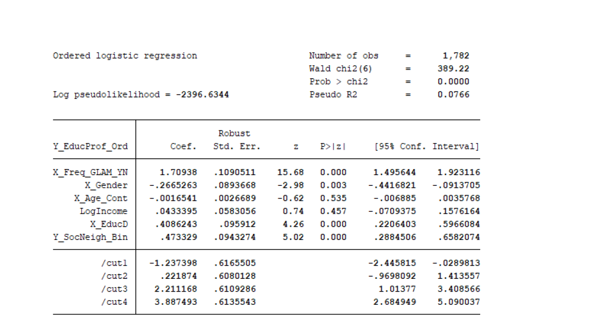
Figure description
Notice in the regression above, that self-reported educational/professional impact of GLAMs is correlated with being a regular GLAMs visitor, education and even gender. However, there is no statistically significant correlation between this variable and log-income nor age as a continuous variable. Although all four dummy variables for educational/professional impact were tested, only the first three are statistically significant, so only these are included.
This result also underscores the relationship between self-reported educational/professional impact of GLAMs and regular GLAMs visitation (three or more annual visits), even after controlling for income and demographic control variables (gender, education and neighbourliness). These educational returns are, in turn, correlated with factors such as neighbourliness (significant with an impact of 0.48 points on 5-point scale). Refer to the main body of the text for a more detailed inquiry into the educational benefits of GLAMs.
Select Regression Results
Overall subjective wellbeing
All GLAMs
The optimal model result for overall subjective wellbeing is determined by the maximum size of the visitation frequency variable coefficient, its statistical significance (p-value <0.05) and minimal standard error. Based on these criteria, the 2SLS instrumental variable regression model performs best. With a visitation frequency (continuous) coefficient of 0.276, each visit to all GLAMs is expected to increase self-reported quality of life measures (on a 0-10 Likert scale) by 0.276 points; a modest yet positive result.
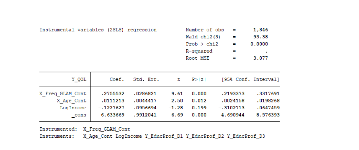
Figure description
We see stronger impacts of visitation frequency on quality of life for individual GLAM types, all with coefficients between 0.6 and 0.9. Although differences between venues are minimal, archives have the greatest impact with a coefficient of 0.880, followed by galleries with 0.717, museums with 0.686, and finally libraries with 0.667. All visitation frequency parameters are statistically significant. Refer to the regression outputs below for details. In cases where income is statistically significant, this was included for monetization purposes and consistency across the variety of models run.
Galleries
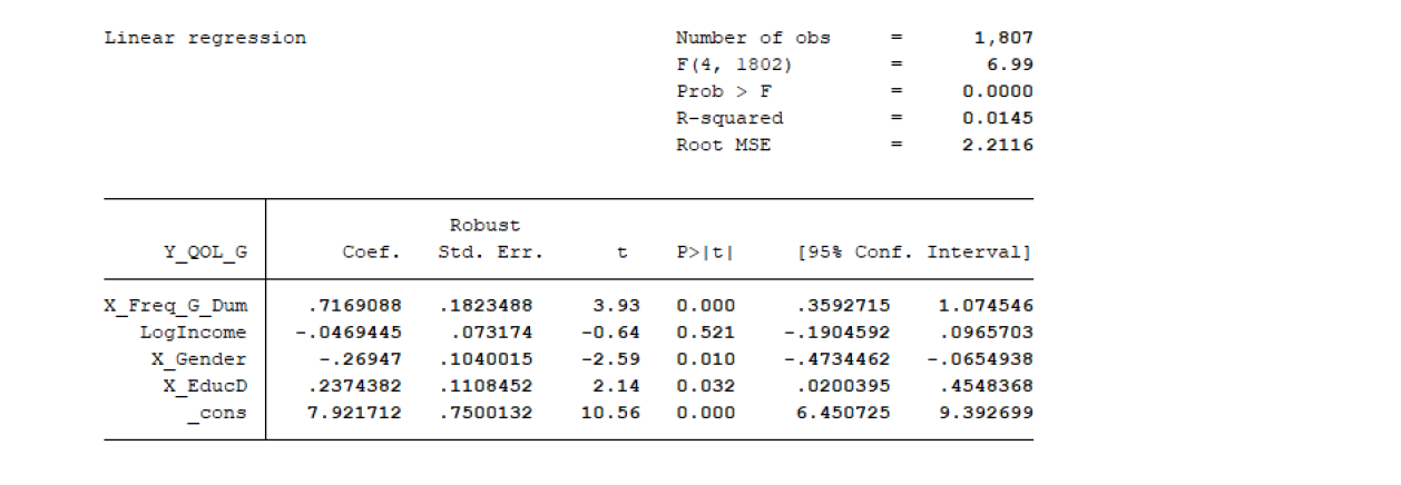
Figure description
Libraries
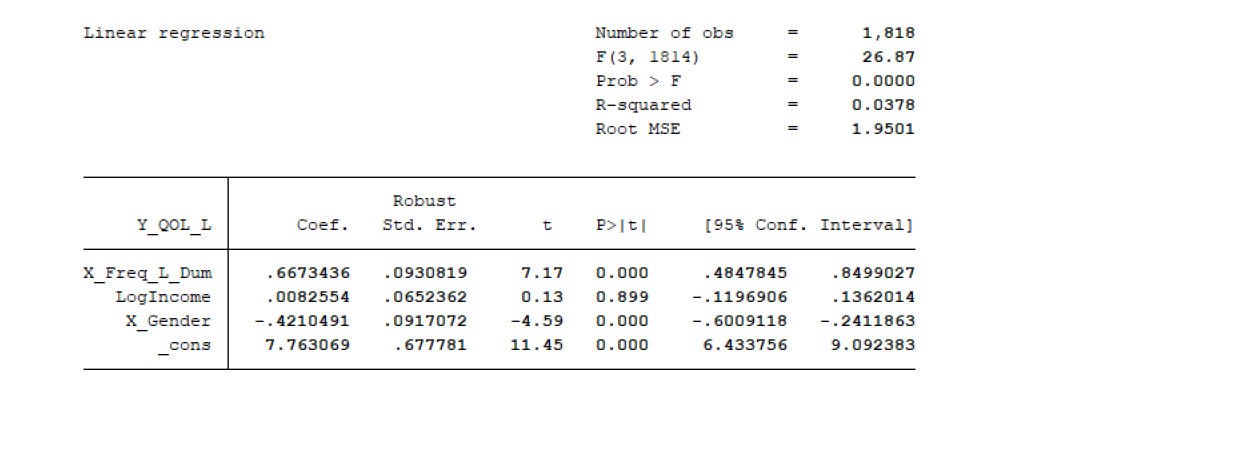
Figure description
Archives
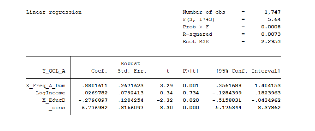
Figure description
Museums
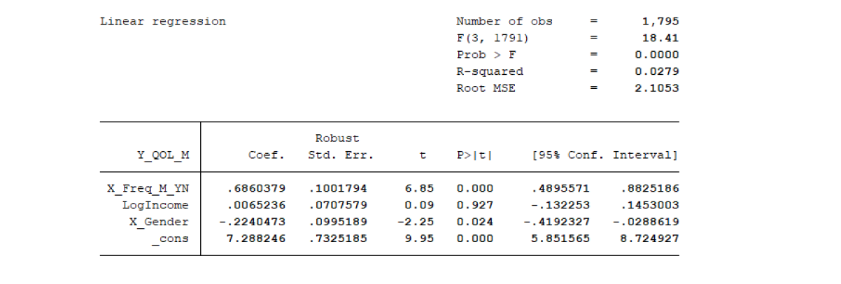
Figure description
Health
All GLAMs
The strongest result for all- GLAMs health benefits is the 2SLS instrumental variable regression, which includes an ordinal dependent variable and a dummy variable for visitation frequency in the second stage regression. The first stage shows that three of the four dummy variables for self-reported educational/professional impact of GLAMs visitation are significant. The errors from this regression are then used in the second stage regression which incorporates age and log of income, both significant. Cross-products between these variables, or interaction terms (age*income, income*education etc.), were tested, but not found to be significant predictors.
Using this two-stage approach, we estimate that regular GLAMs visitors report a 0.4 point increase in self-reported health, on a 1-5 scale, controlling for age, income, and effectively the self-reported educational/professional impact of GLAMs. Notice that income is statistically significant, meaning that the impact of GLAMs visitation on health, controlling for demographic factors, can be monetized (see Section 8.2).
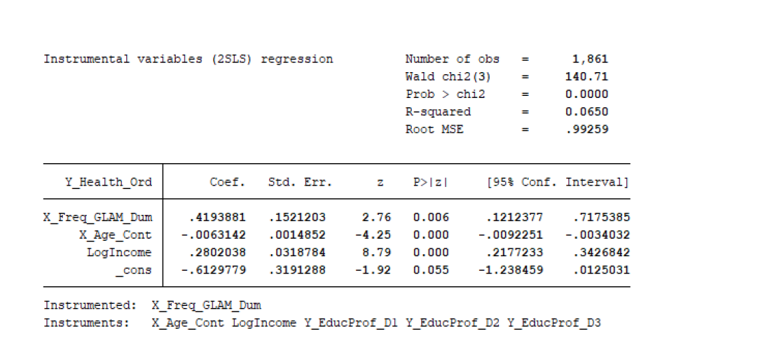
Figure description
For the individual GLAMs, the strongest results were produced using ordered logit regressions, with the exception of libraries, for which a simpler logistic regression (logit) model produced a marginally higher visitation coefficient. Across all models, visitation frequency is captured using a dummy variable (i.e. its coefficient measures the impact of regular visitors, those who visit three or more times annually), as this produced the best results. The preferred model choice makes intuitive sense since self-reported health is measured on an ordinal scale, and the non-linear ordinal logistic regression is designed specifically to meet this purpose.
Galleries show the highest impact with a visitation coefficient of 0.603, meaning that frequent gallery visitors have an estimated 0.603 point higher self-reported health score on a scale from 0-4. Archives show the second highest impact with 0.484, followed by libraries with 0.375 and museums with 0.232 impact factors.
Galleries
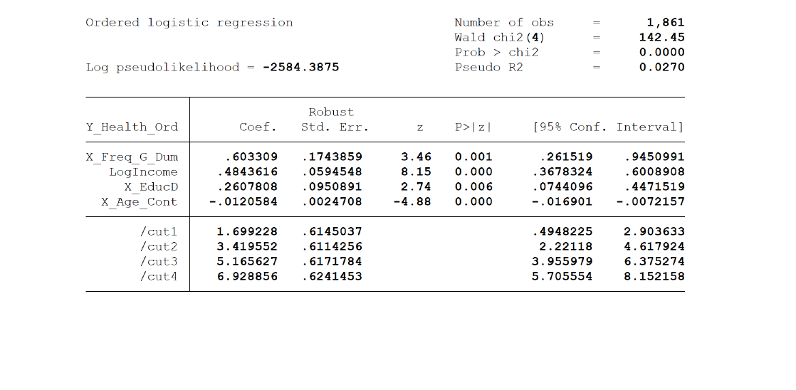
Figure description
Libraries
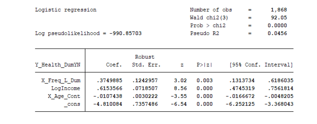
Figure description
Archives
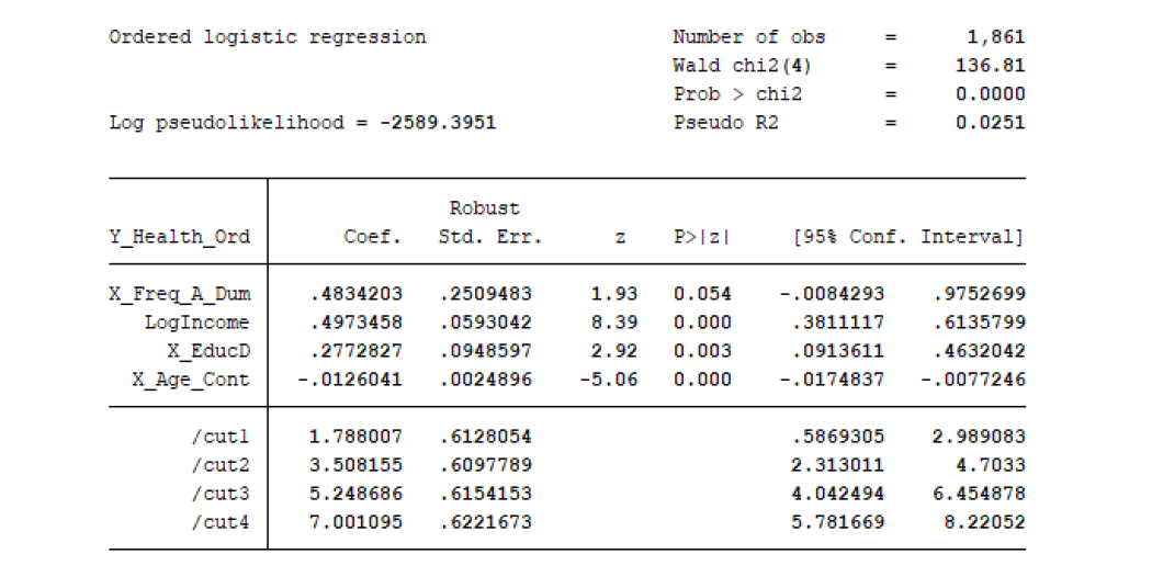
Figure description
Museums
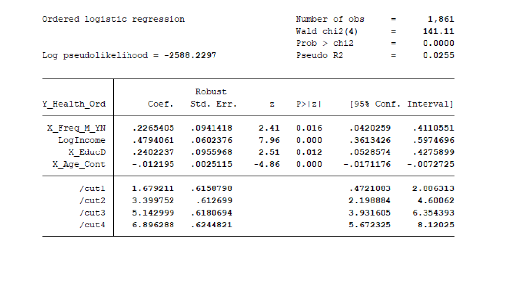
Figure description
Neighbourliness
All GLAMs
Relative to the other subjective wellbeing-related dimensions, GLAMs visitation has a large effect on neighbourliness. Using a logistic regression model, we see a visitation impact or coefficient of 1.054 that is highly significant (p-value of 0.000) and with acceptable robust standard errors (0.281), as shown in the model output below. Since the dependent variable is binary, we do expect the non-linear, logarithmic model to provide a better fit. However, if the visitation coefficient is to be interpreted as the conditional probability that frequent visitors will have high interaction with their neighbours, this gives a probability over 1, which is clearly impossible. This overshooting of the model is caused by an imperfect fit of the regression curve to the data. Yet we can say that there is a very high degree of correlation between frequent visitors and neighbourliness.
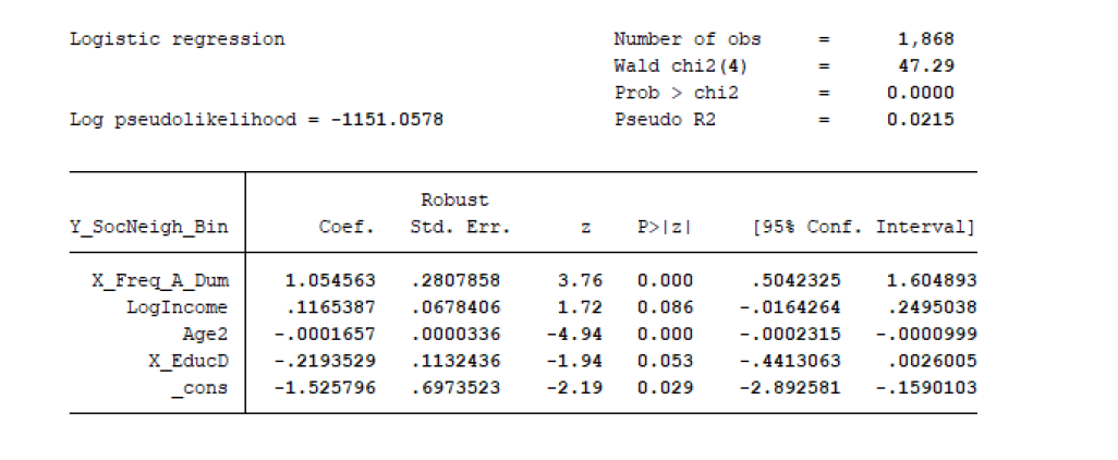
Figure description
Despite estimating a slightly lower frequency coefficient, the 2SLS instrumental variable regression is another important result. This regression involves an ordinal dependent variable and a dummy variable for visitation frequency in the second stage regression. This approach parallels that used for health; indeed, the same variables were found to be significant in both the first stage (self-reported educational/professional impact of GLAMs dummy variables) and the second stage (age and log of income) regressions. Again, interactions between these variables were tested, without significant results. Using this two-stage approach, we estimate that regular GLAMs visitors report a 0.5 point increase in self-reported health, on a 1-5 scale, controlling for age, income and effectively self-reported educational/professional impact of GLAMs.
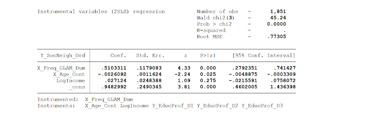
Figure description
For the individual GLAMs, we see an even higher impact factor for archives of 1.250. Given the caveats expressed in the all- GLAMs regression, we can say that those who visit archives are exceedingly likely to know and interact with many of their neighbours. Galleries also show a high impact factor of 0.944. Optimal results for libraries and museums are obtained by ordered logistic regressions, which seem to provide a better fit to the data. Indeed, the logistic regression for libraries did not yield statistically significant results. Regular library visitors are expected to have a 0.167 increase in the probability of associating closely with their neighbours, and regular museum visitors a 0.374 increase in probability.
Galleries
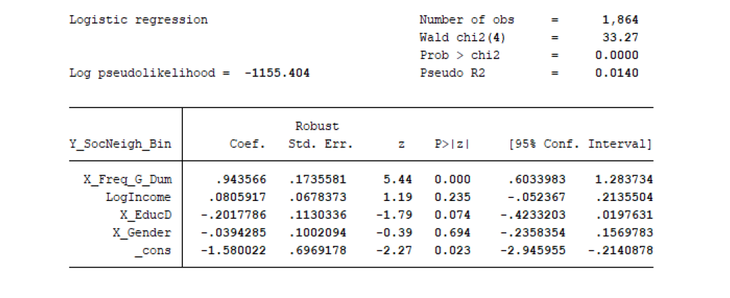
Figure description
Libraries
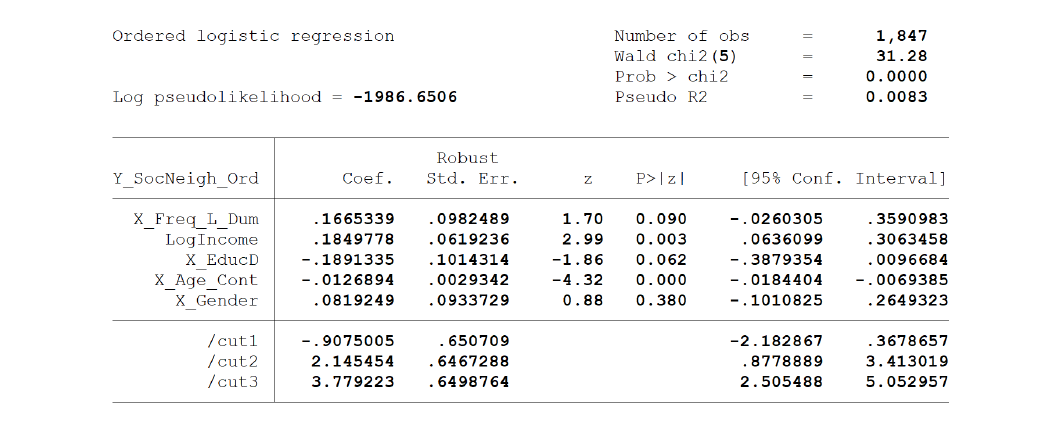
Figure description
Archives
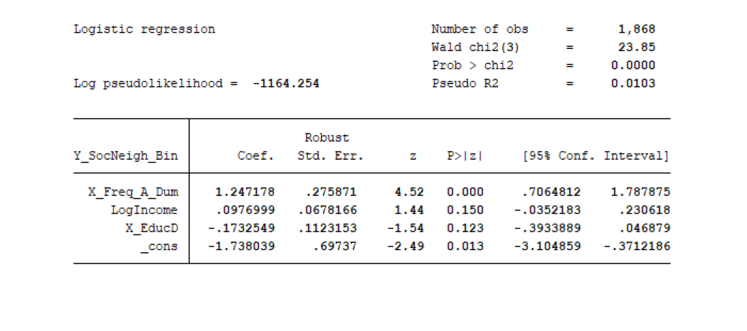
Figure description
Museums
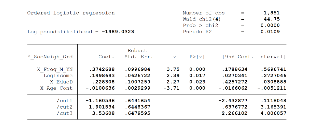
Figure description
Volunteering
All GLAMs
Volunteering also produces a very strong result, with frequent visitors to all GLAMs estimated with 0.983 probability—conditional on consistency in demographic controls of income and education level, both significant—to participate in volunteering and similar community engagement activities. The strength of this result compared to the simple linear regression and 2SLS instrumental variable regression models is no doubt based on the specification of the dependent variable, which is a dummy variable. Interestingly, age has a negative (although very small) coefficient, meaning that people are less likely to volunteer as they age—perhaps a counterintuitive result. Not surprisingly however, education has a strong positive impact, with those having a college degree being 48% more likely to volunteer; a highly significant result with p-value of 0.000.
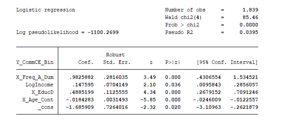
Figure description
We see very high impact factors for the individual GLAMs, especially galleries with 1.195 and archives with 0.983. Since the best models are all logistic regressions with dummy dependent variables, this corresponds to near certainty (approaching or even overshooting conditional probabilities of 1) that being a regular visitor to these venues aligns with volunteering and related community involvement behaviour. The relatively lower results for libraries and museums are still high compared with the other wellbeing aspects considered. Overall, we can conclude that regular GLAMs visitation has a large and significant impact on volunteering.
Galleries
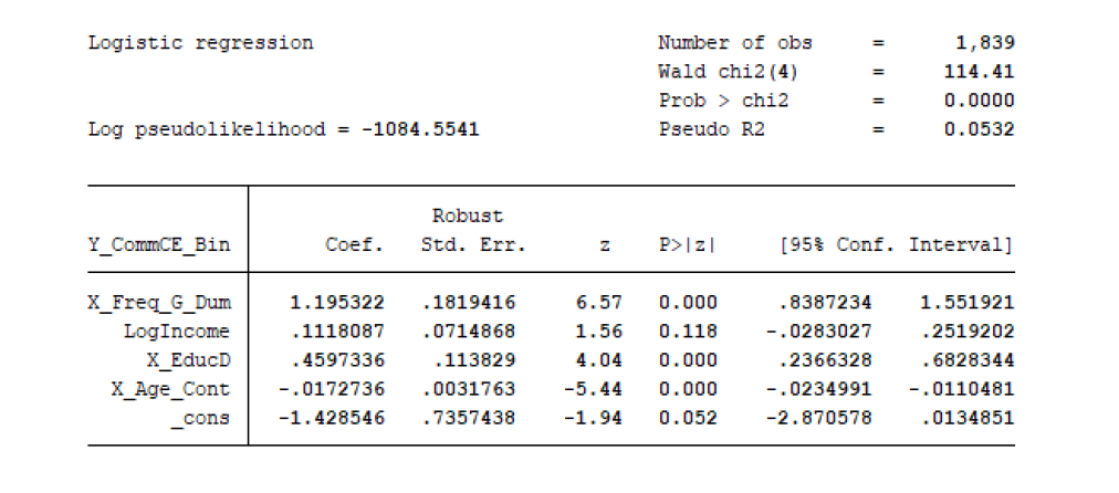
Figure description
Libraries
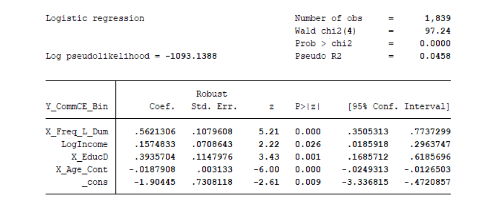
Figure description
Archives
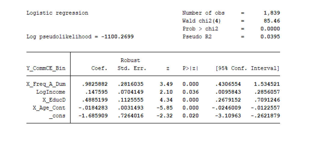
Figure description
Museums
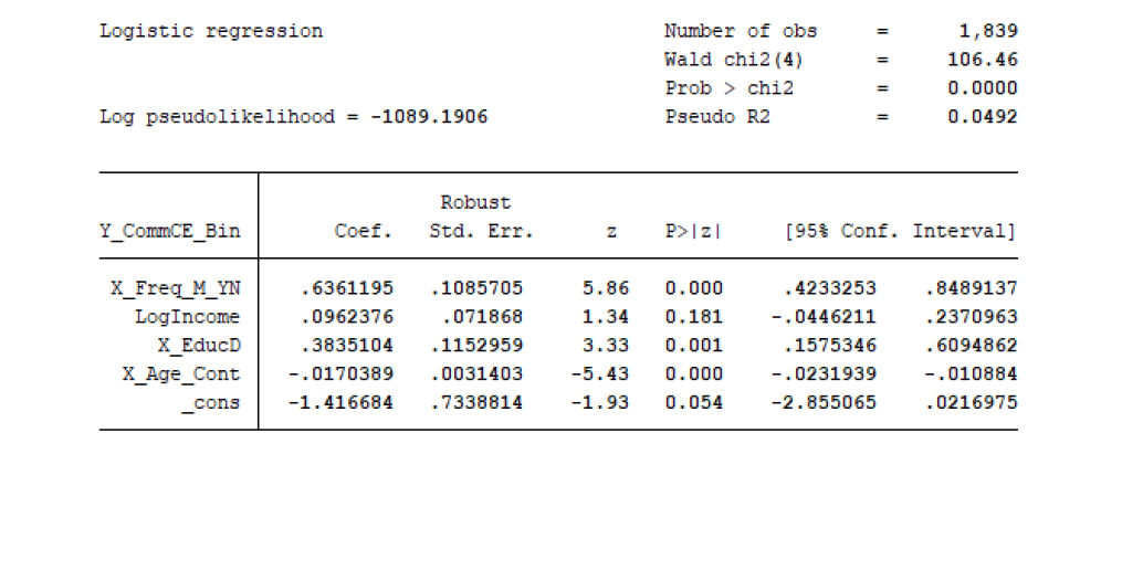
Figure description
Appendix 5 Other Wider Benefits
Background
As indicated in Chapter 8, there are a number of potential wider benefits associated with GLAMs which have been explored in the literature. This appendix provides further details on such benefits.
Social Capital and Informal Education
There is a large volume of evidence that improving key indicators such as literacy is of benefit to society and the economy. For example, recent Canadian work has indicated strong links between literacy and economic growth.Footnote 142 Other past Canadian and international work has had similar findings. However, it should be noted that the authors in question invariably make the point that causal linkages remain an issue.
As indicated above, this study allows for the impacts of formal school education and its interaction with GLAMs. In principle, informal education could also be accounted for within an economic welfare framework. However, an additional challenge with informal education is that, while the returns to formal education are well established, those for informal education rely to varying degrees on additional inferences about causality. For this reason, we are more cautious about the attribution of informal educational benefits to GLAMs.
Nonetheless several studies have attempted to explore such linkages both internationally and within Canada, and the evidence is gradually becoming more compelling. For example, work by Copenhagen Economics (2015) explores the potential link between Danish school children reading books borrowed from public libraries, PISA reading test scores, the likelihood of post-secondary educational entry and higher wages. This work suggests that child usage of public libraries in Denmark could equate to DKK 2.1 billion annually (or $0.4 billion) in economic benefits (expressed as higher education productivity gains).Footnote 143
Fujiwara et al. (2015) examined the probability of tertiary education entry with increased library usage, finding that library visits increase the probability of entering tertiary education, with total benefits equating to £2,113 per person (in 2009 prices).Footnote 144 Detailed Australian work has also shown some linkages between children’s reading activity, PISA reading scores and economic growth, though the evidence is more mixed for effects on long-term wages effects.Footnote 145
In Canada, past work by the OECD has linked student borrowing of books from public or school libraries with PISA scores, both at a national and provincial level.Footnote 146 Other OECD studies focusing on Canada also examine the link between reading, PISA reading scores and the probability of entry to tertiary education.Footnote 147 Past work has also examined the links between public library usage and the literacy scores of Ontario youth, finding a positive relationship between the two using regression analysis.Footnote 148
Some of the most intriguing (and compelling) Canadian research comes from the recent work of Childs et al. (2016) on cultural capital.Footnote 149 These authors look at the frequency of attendance at Canadian cultural venues, including museums and galleries, the incidence of informal reading, PISA scores and the probability of college or university entry. Moreover, this work is especially compelling since it is longitudinal in nature—i.e. it uses recent waves of the Youth in Transition surveys to examine whether those who attended GLAMs and/or undertook more informal reading did actually attend higher education to a greater extent than those who did not. Their work finds that attending an art museum or gallery, an opera, ballet or classical symphony concert, or live theatre increased the probability of university attendance by about 6.6 percentage points for females and 3.4 percentage points for males, while indicating a “love” for reading (reading engagement) increased it by 6 percentage points. As is the case with the other studies above, however, the authors do issue cautions about interpreting these results as causal.
Other recent Canadian research includes the work of Andersen and Jæger (2016). This analysis used relatively sophisticated econometric modelling to find that various forms of cultural capital (including reading) had an impact on Canadian PISA scores, noting that effects were larger for students in more challenging educational environments than those in more privileged ones.Footnote 150
Of course, it may also be that informal education through GLAMs is of importance to adults. Once again there is a large body of evidence in Canada and elsewhere that adult literacy and skills development is correlated with beneficial economic outcomes. Recent Canadian modelling work using adult PIAAC scores, for example, has shown an association between literacy and informal educational attendance.Footnote 151 Other studies have examined links between adult library usage and literacy.Footnote 152 As noted above, literacy in turn has been linked with higher wages and/or economic growth.
However, direct evidence on the specific impact of GLAMs on such adult skills development and wage and economic growth outcomes is more limited. This may be because less interest is shown in adults (compared to children), but also because such work would require longitudinal studies for more solid evidence of effects (i.e. it would require the study of adult GLAM usage and social and economic outcomes over an extended period of years), a point also made by Krupar et al. While some longitudinal work has also been undertaken on adult museum visitation by Falk and Needham, the evidence base remains limited.Footnote 153
For example, it seems logical to assume that adults who are regular museum visitors come away as better educated, more informed and more engaged citizens. Indeed, some of these informal learning outcomes may be reflected in the wellbeing indicator results for health, neighbourliness and volunteering, discussed in the previous appendix. These are important results within the Canadian context as noted above.
Nonetheless, in contrast to younger visitors, there is less evidence on the effects of such informal learning on potential wages and/or economic growth and no comparable quantification of broader effects akin to those developed by authors such as Riddell. The same is true for public libraries; while a variety of studies have noted potential impacts of libraries on adult learning and literacy, comprehensive studies linking public library usage, literacy and growth over time remain rare.Footnote 154
Some of these effects may be included in studies which examine long term “macroeconomic” effects of GLAMs such as libraries. These are discussed below. However, the broad nature of these studies makes it difficult to isolate out what effects are being included.
In short, there have been promising advances in our understanding of the effects of GLAMs on informal education, and some effects could be quantifiable, particularly in the case of informal learning by children and young adults. We have adopted a relatively cautious stance on this issue and excluded these effects from the CBA for this study. Nonetheless, it is important to highlight the ways in which such effects might impact on economic welfare.
Long-term Economic Spillover Effects
As indicated in Section 8.5, one contention is that GLAMs may create long-term spillover effects, which are not captured within conventional economic welfare frameworks.
Note, however that this is no more or less true for GLAMs than for other forms of economic activity. For example, using a conventional framework, the economic benefits (i.e. increase in productivity) from the new metro link, referred to in the main text, would be reflected in the lower costs of the new route and increased business usage of the service. While it may not seem obvious, the conventional framework would actually incorporate the benefits of the new link as they spread out to other business across the economy.Footnote 155
However, it may be that, in time, the increased commercial interaction leads to still greater (and unanticipated) long-run innovation and higher productivity within the economy as a whole, as people develop ideas upon ideas and so on. Like R&D spillovers, perhaps the increased interactions result in inventors coming up with brilliant new ideas, for example. The magnitude of such additional long-term spillover effects would not be captured within a standard economic welfare framework.
Some have therefore argued for alternative “top down” macroeconomic approaches to incorporate such missing spillover effects. Akin to some of the work on literacy described above, these studies look at the relationships between factors such as GLAMs usage and economic growth at the broad national level. This is distinguished from the “bottom up” approach used by economic welfare and in the TCM framework above, where user behaviour is the basis of the assessment. A comparison between the two is indicated in Fig. 47.
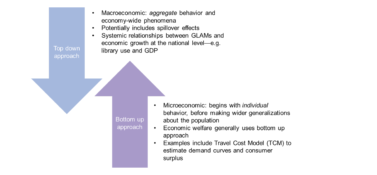
Figure description
However, such approaches are subject to the same critiques as those noted above—they look at broad relationships at the national level and require assumptions about causality. This is in contrast to the known benefits of GLAMs usage using the bottom up economic welfare approaches such as the TCM—i.e. we know that people are using GLAMs and then proceed to measure value on the basis of that usage.
In addition, some (or much) of the assessed benefits of such modelling could be captured by the standard economic welfare approach, so there is a need to be wary of double counting. To date, the standard framework has proved remarkably robust in dealing with the critiques of those who suggest that missing benefits are picked up by top down modelling. This is particularly so in more commonly analyzed areas (such as transportation economics), where economic welfare approaches have been compared to top down ones in detail.Footnote 156 This suggests that such arguments need to be treated with due initial caution.
It is also the case that much GLAMs visitation is not commercial in purpose, which could limit the applicability of spillover arguments.
Nonetheless, it is worth examining the case for economic spillover effects of GLAMs, though these are limited and would mainly appear to relate to the library and archival sectors.
Work by Liu and Skelly, cited above, has examined links between libraries and economic growth using a top down approach. However, the authors of such studies note that causality remains an issue. Other recent top down work has been related to a variety of open data or open government data (OGD) initiatives, which may have implications for the potential spillover benefits of public archives. This work examined the economic value of freeing up government data and making it available to the general public. In essence, freeing up data could allow decisions to be made in a more optimal way, benefiting individuals and society. Conversely, restricting access to data means decisions cannot be made optimally.
Such studies have estimated extremely large economic benefits arising from open data, including $134 billion in the case of Canada.Footnote 157 In addition, arguments have been made that open data initiatives could help support broader social objectives, such as the rule of law, democratic institutions and trust. These are effectively another form of social capital argument.Footnote 158
However, some critiques have been made of the size of such estimations.Footnote 159 In many cases, much of the benefits relate to the sale of commercial data, such as land and/or geospatial data, which may be quite different to the offerings in public archives.Footnote 160 Archives themselves have expressed skepticism along these lines. Responding to a paper exploring the valuation of public sector information (PSI), Australia’s National Archives argued that material from the archives, and material produced by the archives, largely has a social or cultural or evidential value, rather than an economic value.Footnote 161 As the paper states:
The economic value of some types [of data], such as geospatial information can be assessed quite readily. It is less appropriate to attempt to attach a dollar-value to cultural collections.
The archives would support this, emphasizing that the material released by the archives, although it may be used in commercial products, for example, school text books and documentaries, does not in itself generate a significant commercial value in the way that statistical information, spatial data and hydrological data is of immediate commercial use in specific sectors. Therefore, we would assert that for the material published by the archives, the economic value arising from its use is insignificant to the point of being unmeasurable.
However, this may be taking too narrow a view of “economic” value, focused more on measures such as revenue and GDP. As indicated above, economic welfare includes the concepts of consumer surplus and people’s valuation of GLAMs offerings (such as heritage), whether or not a market transaction is involved. So, for example, the TCM and non-use valuations both act as starting points for an economic welfare-based valuation of archival holdings.
Some of the most extensive international quantification work in this area has been undertaken by Houghton, Beagrie and Gruen. These authors also establish a typology of open data value in which geographical information is of highest commercial re-use value and public archives are the lowest. Nonetheless, they stress that the typology is not exact in all cases and that institutions such as archives can have more value than those seemingly higher up the “value chain.”Footnote 162 Beagrie and Houghton examine a number of digital repositories in the UK, in particular, using both conventional economic welfare approaches and a top down economic modelling approach. Their work suggests benefit cost ratios of 3.0-4.9 for the UK’s Economic and Social Data Service ( ESDS) using economic welfare approaches, but up to 10 using a top down macroeconomic approach.Footnote 163 However, apart from the usual caveats on causality, the extent to which such results would apply to mainstream public archives in Canada or elsewhere is unclear.
In short, there may be an in principle case for GLAMs spillover benefits, as indicated by the example box in the main text, which underlines the broader importance of archival research. However, the lack of strong and comprehensive evidence across GLAMs to date does not allow for a full quantification of such effects.
Employment and Multiplier Effects
Employment
As indicated in the main text, some GLAMs such as libraries may be of great assistance in helping their visitors research jobs and/or in helping the unemployed search for new employment. However, as discussed, it is important not to confuse economic welfare measures with economic impacts. Under an economic welfare approach, there is a working assumption of full employment. This means that a person already in employment getting a new job is not a benefit in the strict economic sense, as the person has simply transferred from one job to another.
However, an unemployed person getting a job would be generally considered a benefit. That person is currently underutilized from an economic perspective and would now be getting a job and earning a wage (to say nothing of the positive psychological effects of employment, which are increasingly recognized). To the extent GLAMs help this process, that could count as a benefit.
In practice, it is challenging to quantify the role of libraries in unemployment assistance; while wages would represent an economic benefit, a key issue would be whether the new role was permanent.
Another issue would be how much of a role the library played among other factors in getting the new job. Indeed, conventional “welfare to work” studies often deal with similar issues.
However, the issue of economic measurement should also be distinguished from that of practical significance. An unemployed person who successfully uses a library to attend training courses and/or research jobs would doubtless view it as a positive outcome, regardless of the technicalities of measurement.
Multipliers
The presence of GLAMs may provide a boost to businesses such as local retailers. For example, consider the opening of a new gallery in a local area. This could provide a boost to local retailers, which in turn buy from suppliers, who in turn buy from theirs and so on, creating multiplier effects across the local area. Should these effects be included in a GLAMs cost-benefit analysis?
These effects would be the type of impacts captured by an economic impact analysis. As noted above, economic welfare should not be confused with economic impact analysis. Economic impact analysis measures the amount of economic activity an initiative might bring—e.g. a new library might create jobs and boost GDP through spending. However economic welfare frameworks measure a different set of metrics and use a different starting point. Economic impact studies measure economic activity in terms of contributions to the economy as a whole, or the share of the “economic pie” accounted for by institutions such as GLAMs. By comparison, economic welfare studies measure how society is better off in terms of net benefits (benefits less costs), i.e. how institutions such as GLAMs grow the “economic pie”.
In the example above, a retailer might obtain higher revenues from the presence of a GLAM. However, economic welfare analysis focusses on net benefits—so it is profits rather than revenues which would be of relevance. Moreover, the conventional economic welfare framework may in fact capture many of these transmitted benefits, so adding multiplier effects could be double counting. For these and many other technical reasons, multiplier effects on local businesses are generally excluded from an economic welfare framework, unless there are very specific circumstances. This is the approach taken in this study. This is consistent with the guidelines issued by the Treasury Board of Canada (which notes that such “secondary market” effects must be excluded from cost-benefit analysis) and the analysis offered in standard economic texts.Footnote 164
As indicated, this does not mean economic impact or economic welfare are the "right” or “wrong” answer to measuring the value of GLAMs. For example, an alternative approach to measuring the economic effects of the gallery would be to define the local area as the clear (and only) area of interest and to use an economic impact approach to assess the GDP and jobs generated in that area. This would produce an alternative viewpoint on galleries’ benefits (i.e. one focused on benefits as conventionally measured by markets). However, just as it would be incorrect to add multiplier effects to a welfare framework, so consumer surplus and non-use value cannot be added to an economic impact one—they measure different things. Neither answer is necessarily “better.” However, the key point is for analysts to be aware of the framework and scope of the analysis they wish to undertake and to be consistent with that framework.
Appendix 6 Questionnaire
National Survey
The Canadian Museums Association ( CMA), on behalf of the Ottawa Declaration Working Group, is undertaking work with Oxford Economics to quantify how galleries, libraries, archives, and museums ( GLAMs) contribute to the Canadian economy, as well as more broadly to society. In order to do this, it is important for us to understand how the general public views these institutions.
Throughout this survey we will ask you a series of questions about the following institutions:
- Non-profit, public galleries whose primary purpose is communication rather than selling;
- Non-profit, public libraries in municipalities and regions, Indigenous libraries, academic libraries at Canadian post-secondary institutions, special libraries (for example, in hospitals, museums, galleries, botanical gardens, as well as serving people with disabilities) and provincial, territorial and national libraries;
- Non-profit, public archives in municipalities and regions, Indigenous archives, archives at Canadian post-secondary institutions, and provincial, territorial and national archives; and
- Non-profit, public museums in municipalities and regions, Indigenous museums, and museums at Canadian post-secondary institutions.
Please DO NOT answer the questionnaire in relation to any institutions that are profit-focused (i.e. those that exist for the sole purpose of generating revenue through buying and selling cultural collections).
We appreciate you taking the time to complete this survey. It will only take a few minutes and all responses will be treated as confidential.
Quota questions (1 min)
A1 First official language spoken
- French - 1 (administer French questionnaire)
- English - 2 (administer English questionnaire)
- Other - 3 (ask to choose preferred language for questionnaire between English and French)
A2 In which Province or Territory do you have your permanent residence?
- Alberta - 1
- British Columbia - 2
- Manitoba - 3
- New Brunswick - 4
- Newfoundland and Labrador - 5
- Northwest Territories - 6
- Nova Scotia - 7
- Nunavut - 8
- Ontario - 9
- Prince Edward Island - 10
- Quebec - 11
- Saskatchewan - 12
- Yukon - 13
A3 What is your Postal Code?
- FREEFORM
A4 What is your gender?
- FREEFORM
- Male - 1
- Female - 2
- Other - 3
A5 What is your age?
- 15-19 - 1
- 20-24 - 2
- 25-34 - 3
- 35-44 - 4
- 45-54 - 5
- 55-64 - 6
- 65+ - 7
A6 What is the highest educational level you have completed?
- No certificate, diploma or degree - 1
- High school diploma - 2
- Apprenticeship or other trades certificate - 3
- College diploma or university below bachelor's - 4
- Bachelor's degree - 5
- Postgraduate - 6
- Other (please specify) - 7
User/non-user split (1 min)
B1 Have you visited the following venues?
Galleries (these could range in size from major ones such as Art Gallery of Nova Scotia, Art Gallery of Ontario, etc. to smaller local ones.)
- Yes, I have visited a gallery within the last 12 months - 1
- Yes, I have visited a gallery, but it was more than 12 months ago - 2
- No, I have never visited a gallery - 3
Libraries (these could range in size from large urban ones such as Toronto Public Library, La Grande Bibliothèque, Ottawa Public Library, etc. to smaller local ones and specialist ones such as academic libraries and special libraries - e.g., in hospitals, museums, galleries and those serving people with disabilities.)
- Yes, I have visited a library within the last 12 months - 1
- Yes, I have visited a library, but it was more than 12 months ago - 2
- No, I have never visited a library - 3
Archives (these could range in size from Archives de Montréal, Archives of Ontario, etc. to smaller local ones, like the archives at the Whyte Museum of the Canadian Rockies in Banff.)
- Yes, I have visited an archive within the last 12 months - 1
- Yes, I have visited an archive, but it was more than 12 months ago - 2
- No, I have never visited an archive - 3
Museums (these could range in size from Royal Ontario Museum, Royal BC Museum, Royal Tyrrell Museum, etc. to smaller local ones, like the Reynolds-Alberta Museum.)
- Yes, I have visited a museum within the last 12 months - 1
- Yes, I have visited a museum, but it was more than 12 months ago - 2
- No, I have never visited a museum - 3
Users (3-4 mins)
You’ve indicated you visited a gallery, library, archive or museum within the last 12 months.
C1 How many visits did you make to GLAMs over the past 12 months? (Enter numbers for each category where relevant)
Galleries
- 0 - 1
- 1-2 - 2
- 3-4 - 3
- 5-6 - 4
- More than 6 (please specify how many) - 5
Libraries
- 0 - 1
- 1-2 - 2
- 3-4 - 3
- 5-6 - 4
- More than 6 (please specify how many) - 5
Archives
- 0 - 1
- 1-2 - 2
- 3-4 - 3
- 5-6 - 4
- More than 6 (please specify how many) - 5
Museums
- 0 - 1
- 1-2 - 2
- 3-4 - 3
- 5-6 - 4
- More than 6 (please specify how many) - 5
And now to help understand your usage a bit better, we’d just like to ask you a few more questions about your last trip to a gallery, library, archive or museum.
C2 Considering for a moment your last trip to a GLAM, was it to a:
- Gallery - 1
- Library - 2
- Archive - 3
- Museum - 4
- Don’t know - 5
C3 And do you remember the name of the GLAM you visited on that last trip? If so, please enter it below (free text). If you can’t remember please go to the next question.
FREE TEXT RESPONSE (NON-MANDATORY)
C4 And how you did you get there on that trip?
- Walk - 1
- Drive - 2
- Public Transportation - 3
- Taxi/Uber or other ridesharing - 4
- Airplane - 5
- Train - 6
- Bike - 7
- Other (please specify) - 8
- Don’t know - 9
C5 And on that last trip, how much time did it take to get there (as a one-way trip)? Just give your best estimate.
- Less than 5 minutes - 1
- 5-9 minutes - 2
- 10-19 minutes - 3
- 20-29 minutes - 4
- 30-59 minutes - 5
- 60-90 minutes - 6
- More than 90 minutes (please specify how long) - 7
- Don’t know - 8
C6 How long did you spend there on your last visit? Just give your best estimate.
- Less than 30 minutes - 1
- 30 minutes to an hour - 2
- 1 to 2 hours - 3
- 2 to 3 hours - 4
- 3 to 4 hours - 5
- 4 to 5 hours - 6
- 5 to 6 hours - 7
- Over 6 hours - 8
- Don’t know - 9
C7 And finally on travel, how much did you spend to get there on your last trip (as a one-way trip)? Include travel costs such as fares, gasoline and parking if relevant. Just give your best estimate.
- $0 - 1
- $1-5 - 2
- $5-10 - 3
- $10-15 - 4
- $15-20 - 5
- $20-80 - 6
- $80-140 - 7
- $140-200 - 8
- More than $200 (please specify how much) - 9
- Don’t know - 10
Willingness to pay (4-5 mins)
The following questions are designed to help us capture the value that you place on galleries, libraries, archives and museums and on the services they provide. These questions are not an indication that current funding arrangements will change.
Galleries, libraries, archives and museums have traditionally been important contributors to Canadian society. They have also been broadening their services through providing Internet access, community gathering spaces, educational opportunities, maker spaces, programming for marginalized community members and many other services. In so doing, the sector aims to further extend its social impacts.
D1 In one way or another, all Canadians currently pay towards the annual upkeep and development of galleries, libraries, archives and museums ( GLAMs) whether through taxes, donations, entry fees or other means.
However, imagine that GLAMs had no other sources of government or private funding and the only way of maintaining them was to rely on individual donations.
In such a situation, what is the maximum amount you would be willing to pay each year as a donation to maintain all of Canada’s non-profit GLAMs?
In answering this question:
- remember that your donation is for all non-profit Canadian GLAMs across the whole country, not just your local one(s);
- try to be as honest as possible in your response; and
- remember that you must also meet your other everyday costs of living.
You can either choose one of the amounts indicated below OR provide an amount in the "Other amount (please specify) $" field below.
Note that you must select the maximum amount you would donate to each one of the institutions (i.e. one for galleries, one for libraries, one for archives and one for museums). These will add up to a total amount that will represent the total maximum amount you are willing to pay for Canadian non-profit GLAMs as a whole.
(RESPONSE REQUIRED FOR EACH TYPLE OF GLAM)
| Canadian galleries: (Maximum amount you are willing to pay each year $) | Canadian libraries: (Maximum amount you are willing to pay each year $) | Canadian archives: (Maximum amount you are willing to pay each year $) | Canadian museums: (Maximum amount you are willing to pay each year $) |
|---|---|---|---|
| $0 | $0 | $0 | $0 |
| $10 | $10 | $10 | $10 |
| $20 | $20 | $20 | $20 |
| $30 | $30 | $30 | $30 |
| $40 | $40 | $40 | $40 |
| $50 | $50 | $50 | $50 |
| $75 | $75 | $75 | $75 |
| $100 | $100 | $100 | $100 |
| $150 | $150 | $150 | $150 |
| Other amount (please specify) | Other amount (please specify) | Other amount (please specify) | Other amount (please specify) |
D2 What is the basis for the answers you give when you were asked to value GLAMs? Please select all that apply.
MULTIPLE RESPONSES PERMITTED
- I value GLAMs highly - 1
- I am happy to fund GLAMs - 2
- I have never used (or I am unlikely to use) some (or all) GLAMs - 3
- I object to funding GLAMs - 4
- I can't afford to pay - 5
- I do not value GLAMs - 6
- Other (please specify) - 7
Qualitative analysis (4-5 mins)
Galleries, libraries, archives and museums (GLAMs) make a broader contribution to Canadian society in many ways that can’t be measured through dollars and cents. For this reason, it is also important to get a broader idea of people’s thoughts and feelings about Canadian GLAMs.
The following questions ask you to consider some of these broader values.
E1 Please rate (on a scale of 1-10) how important you think the role of each institution is in contributing to the key social objectives below, where 1 is “Not important at all” and 10 is “Extremely important.”
Give a higher rating if you feel the institution makes an important contribution to a social objective and a lower one if you feel it makes a less important one.
Remember that your response relates to Canadian GLAMs across the nation as a whole, not just your local one(s).
Please provide your ratings for each institution in the boxes below. If you feel you don’t know, or can’t say, how important the institution’s contribution to these objectives is, you may click the “don’t know” box.
RESPONSE REQUIRED FOR EACH TYPE OF GLAM, HOWEVER CLICKING THE DON’T KNOW BOX IS ACCEPTABLE.
- Not important at all - 1
- 2
- 3
- 4
- 5
- 6
- 7
- 8
- 9
- Extremely important - 10
| Social objective | Institution | |||
|---|---|---|---|---|
| Community engagement and civic participation | ||||
| Preserving cultural and historical heritage | ||||
| Providing access to resources for research, innovation and education | ||||
| Protection of truth, integrity and social values | ||||
| Quality of life, mental and physical health and wellbeing | ||||
| Providing inspiration for creativity | ||||
| Nurturing of identity for marginalized communities, contributing to community cohesion | ||||
E2 To what extent would you say that you have benefitted from using GLAMs’ resources in your education, or your professional or personal development?
- Not at all - 1
- Not very much - 2
- Moderately - 3
- Very much - 4
- Extremely - 5
- Don’t know - 6
E3 If you have any other comments on why galleries, libraries, archives and museums may or may not have value to you, please feel free to provide them below:
FREEFORM, NON-MANDATORY
Online usage (3-4 mins)
F1 Please indicate if you have used any of the following online channels to access Canadian galleries, libraries, archives or museums (GLAMs) content within the last 12 months. Select all online channels and institutions that you have used.
Ignore those channels you have not used. If you have not used any of these channels, you may select the last check box in each column.
For each channel you select, an open box will appear. Please provide an estimate in that box of how many minutes you think you spent online the last time you accessed the institution (i.e. the length of your last “online session” with that institution).
| Channel | Institution | |||
|---|---|---|---|---|
| Galleries | Libraries | Archives | Museums | |
| Official Website | 1 | 1 | 1 | 1 |
| Online Catalogue | 2 | 2 | 2 | 2 |
| 3 | 3 | 3 | 3 | |
| 4 | 4 | 4 | 4 | |
| 5 | 5 | 5 | 5 | |
| Flickr | 6 | 6 | 6 | 6 |
| Podcast | 7 | 7 | 7 | 7 |
| Mobile apps | 8 | 8 | 8 | 8 |
| Blog | 9 | 9 | 9 | 9 |
| Crowdsourcing | 10 | 10 | 10 | 10 |
| Other online channel | 11 | 11 | 11 | 11 |
| Don’t know | 12 | 12 | 12 | 12 |
| I have not used any of these channels to access this institution within the last 12 months | 13 | 13 | 13 | 13 |
More about you (3 min)
G1 Which of the following best describes your current employment situation?
- Full time employment - 1
- Part time employment - 2
- Self-employed - 3
- Looking after family - 4
- Student - 5
- Unemployed - 6
- Retired - 7
- Long term illness - 8
- Other (please specify) - 9
- Prefer not to say - 10
G2 Which income bracket best describes your individual gross income (before tax) over the past year? Include all sources of income (wage/salary, pensions etc.)
- Less than $25,000 - 1
- $25,001 - $50,000 - 2
- $50,001- $75,000 - 3
- $75,001 - $100,000 - 4
- $100,001 - $200,000 - 5
- Over $200,000 - 6
- Prefer not to say - 7
G3 Do you identify as any of the following?
MULTIPLE RESPONSES ALLOWED
- Indigenous person - 1
- Person with disability - 2
- Member of a visible minority - 3
- Newcomer to Canada (immigrant or refugee) - 4
- Prefer not to say - 5
- None of the above - 6
G4 In the past 12 months, did you do unpaid volunteer work for any organization?
- Yes - 1
- No - 2
- Prefer not to say - 3
G5 Would you say that you know most, many, a few or none of the people in your neighbourhood?
- Most - 1
- Many - 2
- A few - 3
- None - 4
- Prefer not to say - 5
G6 How do you feel about your life as a whole right now?
- Very dissatisfied - 1
- Dissatisfied - 2
- Neither satisfied nor dissatisfied - 3
- Satisfied - 4
- Very satisfied - 5
- Prefer not to say - 6
G7 In general, would you say your health is:
- Excellent - 1
- Very good - 2
- Good - 3
- Fair - 4
- Poor - 5
- Prefer not to say - 6
G8 Thinking about the amount of stress in your life, would you say that most days are:
- Not at all stressful - 1
- Not very stressful - 2
- bit stressful - 3
- Quite a bit stressful - 4
- Extremely stressful - 5
- Prefer not to say - 6
Appendix 7 Descriptive Statistics on Questionnaire
Oxford Economics surveyed 2,045 Canadian residents during the Spring of 2019. To ensure all segments of the Canadian population were being accounted for, we adopted a quota sampling approach along the following dimensions:
- Gender;Footnote 165
- Age band (as illustrated in Fig. 48);Footnote 166
- Official language spoken (23% French and 77% English);Footnote 167
- Highest educational attainment;Footnote 168 and
- Province and territory (as illustrated in Fig. 49).Footnote 169
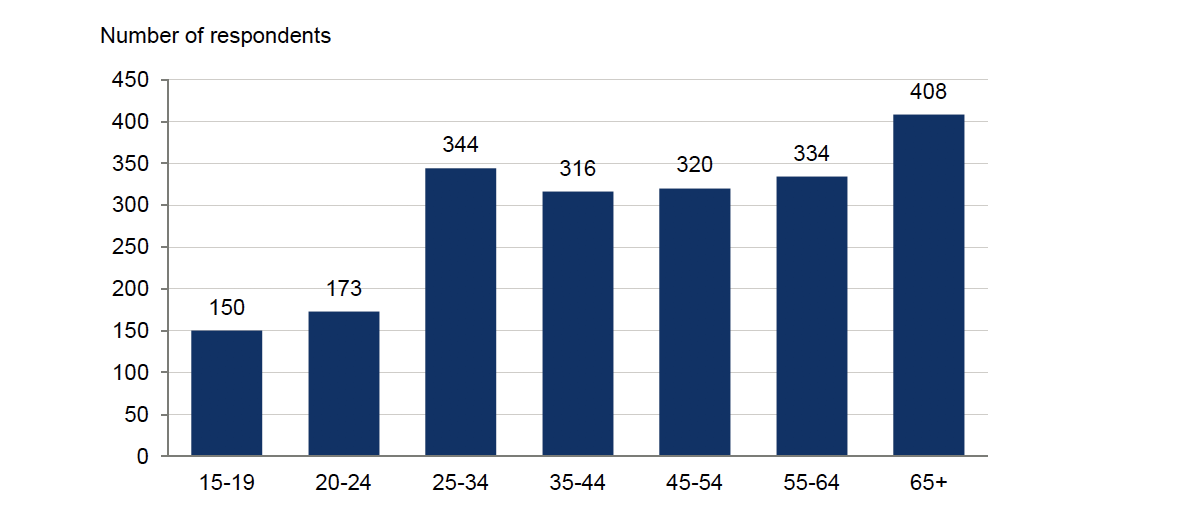
Figure description
Source: Oxford Economics
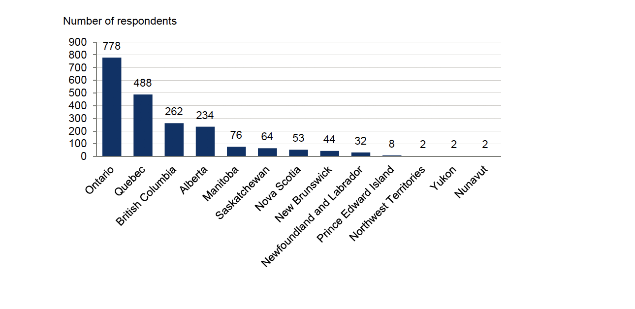
Figure description
Source: Oxford Economics